Pattern Formation in Mathematics

Pattern Formation in Mathematics
Visualization of the dynamics of simple equations
In a plane defined by two independent variables (x, y) a manifold of differently distributed point series can be generated by the repeated application of simple
nonlinear equations. An example for such equations is xn+1 = a xn (1-xn-yn) and yn+1 = a xnyn, n=1,2,3, ..., which simulates a simplified predator-prey system. After a transition process a finite number of points repeating in a cyclic manner may result (periodic attractor). But the points may also move around on an area of the plane chaotically, i.e. in an unpredictable sequence (chaotic attractor). The unpredictability is caused by the exponential growth of small perturbations which are unavoidable in any real process. In much the same way, laws of physics ruling our weather make long term weather forecasts impossible. The growth of perturbations is described by the so-called Lyapunov exponent, which is positive for chaotic and negative for periodic attractors. Pictures M1 through M4 show examples of attractors on the plane and of transitions leading to them.
In pictures M5 through M14 the behavior of the equation xn+1 = r xn (1-xn) is displayed. This equation can be used for the simulation of insect populations or epidemics, r being a parameter describing the environmental conditions. These conditions are here assumed to vary periodically by letting r cycle in different ways between two values A and B. The Lyapunov exponent is indicated on the A-B-plane by different colors.
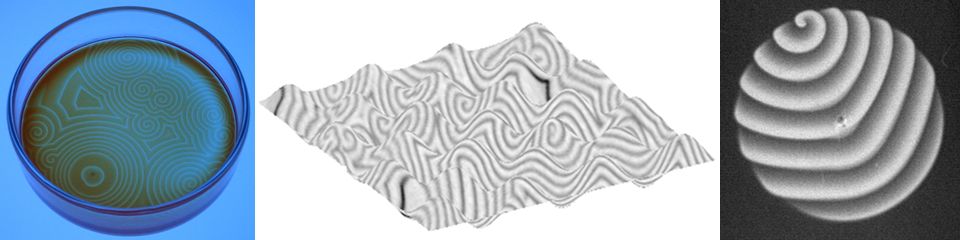
The pattern in picture M15 was generated by dividing the plane into cells. According to simple rules, the state of each cell was determined from the previous state of the cell itself and its neighbors. Patterns similar to those in this picture are observed in nature, e.g. in the experiments shown in pictures C1, C2 and some of the following images.
The selection of pictures presented on the following pages demonstrates that systems with complex behavior in time and space are not necessarily based on complex laws of interaction. It is solely the nonlinearity and the repeated application of these laws which confers beauty and variety to these systems.
Mario Markus


Pictures M1 and M2 show chaotic attractors according to a formula by I. Gumowski and C. Mira, which consists of quotients of polynomials. The variation of parameters leads to a manifold of patterns like the “three-winged” (M1) or the “seven-winged bird” (M2). The repeated application of the formula renders points which move around unpredictably. Only large numbers of such points form organized structures, as shown here.


The coordinates of the images M3 and M4 are given by the concentrations of chemical substances. M3 shows the transition to a periodic attractor. The points calculated first are colored blue, those computed last are yellow. M4 shows the transition to a chaotic attractor (“ocean” in the lower part). Here, points are traced which initially lie within a rectangle. The content of the rectangle assumes the shape of “mountains,” which descend further and further, until they get “caught” by the attractor at the bottom.


An astonishing example of complex temporal phenomena is the so-called logistic equation xn+1 = r xn(1-xn). In spite of its simple form, this equation shows a great variety in its dynamic behavior. For r < 3.57, the xn-series are periodic. For r ≥3.57, however, the series are chaotic, except for some intervals of r which are called “periodic windows.” In pictures M5 and M6, the behavior of the logistic equation for periodically varying r is displayed. The colors in this picture (as well as in the following) represent the Lyapunov exponent λ as a function of A (abscissa) and B (ordinate). When λ changes from negative values to zero, the color changes from blue to white; when λ changes from zero to positive values, the color changes from black to blue.
The r-sequence in pictures M5 and M6 is given by ABABAB... The case r = A = B ("classic" logistic equation) corresponds to the diagonal from the lower left to the upper right corner. Picture M5 shows the neighborhood of a periodic window (period 3). The asymmetry properties of the system with respect to the diagonal indicate that the sequences ABABAB... and BABABA... are not equivalent. Picture M6 is an enlarged detail of picture M5. At smaller scales, structures become visible which are similar to the large-scale picture. The procedure of enlarging and rediscovering structures can be continued indefinitely, thus defining a so-called "selfsimilar object," or a "fractal." Within certain ranges of enlargement, many natural objects have a fractal structure: trees, cauliflower, blood-vessel systems, the rings of Saturn...

Picture M7 shows the environment of the window with period 3 of the r-sequence AABAB AABAB AABAB... The window is the same as in image M5, but here a different r-sequence was chosen. A small change in the sequence - in this case the repetition of A after every other B - has dramatic consequences: a typical of nonlinear systems.

Here, we see a detail of the A-B-plane for the r-sequence AAABB AAABB AAABB... To emphasize certain values of the Lyapunov exponent λ, lines of equal λ's are drawn in white; in between, the color changes from black to goldgreen and back to black as λ increases. Positive λ are shown in dark green (background).

Picture M9: Lyapunov exponent for the r-sequence AAAAAABBBBBB AAAAAABBBBBB ... In those areas where two or more branches overlap two (or more) attractors coexist. (Note such areas in the other images of λ, too.) The coexistence of attractors means, that depending on the initial condition( value of x1) one or another attractor will be reached.

Picture M10 shows a different detail of the A-B-plane for the same r-sequence as in M7. Three branches overlap slightly to the right and below the center. Five branches overlap at the center of the right margin. In these areas three and five attractors coexist, respectively. The branch covering other branches corresponds to the attractor which is reached with the particular initial value chosen here (x1 = 0.5).


Pictures M11 through M13 show further representations of the Lyapunov exponent λ as a function of A and B. As λ changes from negative to positive values, color changes from black to blue, and via white back to blue. The images show that order (i.e. periodicity: λ < 0) and chaos (λ > 0) lie very close to each other in highly "fuzzy" structures. The r-sequences are:
ABAABBAAABBB ABAABBAAABBB ... for M11 BBBBBBBBBBBBA BBBBBBBBBBBBA ... or M12 AAAAABBBBB AAAAABBBBB ... for M13

Picture M14: Lyapunov exponent λ for the r-sequence AABABAB AABABAB... When 4 increases from negative values to zero, color changes from black to yellow. Positive λ (chaos) are shown in blue. The dark curves within the yellow areas represent particularly stable ("superstable") periodical processes. (Note the superstable curves in pictures M5 through M13). Superstable periodicity provides the internal clock of biological organisms with a useful insensibility against perturbations. It is interesting to note the recurring "motif" of picture M5 (top right in M14), now appearing twice and with three overlapping branches (coexistence of three attractors). Close to the center at the right margin, seven branches overlap (coexistence of seven attractors).

A result of the mathematical modelling of a heterogeneously catalyzed reaction, namely the oxidation of carbon monoxide in presence of palladium, is shown in image M15. A cellular automaton describes the chemical mechanisms as a simple process of infection between neighboring cells. The different colors indicate the state of the cells. Due to interactions between cells, spatial structures, like spirals, develop spontaneously from completely unordered states: an example of self-organization, as it occurs in many chemical and biological processes. Picture C2 shows a chemical experiment, in which similar spiral waves are observed. Picture M15 was made in cooperation with Heike Schuster during her stay with us.